胶体在水中的模拟
教程来源:Colloidal
forces | MD Simulation Techniques and Applications (psu.edu)
水中的胶体粒子可以通过多种可能的力进行相互作用,包括范德华力、库仑相互作用、氢键相互作用等。周围的溶质也会影响相互作用势能。要了解有无溶质的势能依赖性,以及胶体颗粒之间的吸引或排斥关系,不同分离距离的平均力势
(PMF)
是我们要研究的关键因素。通过保持粒子相对于不同的相对距离,我们可以了解胶体耗尽力的潜在趋势。
可以使用Gromacs考察不同离子以及它们浓度对胶体粒子之间作用力的影响。
在此体系中,仅探讨空心球状粒子C240。模拟的具体参数:恒定体积(4*4*6
nm3 ),温度 300K。
因篇幅问题,溶质离子为1
M的铵根离子(NH4 + )和硝酸根离子(NO3 - )的情况暂不讨论,读者可以在构建完体系之后,使用gmx solvate命令将水替换为溶质粒子,并修改topol文件即可。
体系搭建
体系包括了两个空心的C240球溶解于水中。从文献中可知,C240的直径为1.5
nm。因此为了选取两个C240之间的相互作用,模拟盒子选取为4*4*6。
为了防止水被添加到C240球内,两个dummy原子被放在C240中心(gmx insert-molecule)。
然后溶剂化体系(排斥半径为0.75
nm,gmx solvate -radius 0.75)。
使用gmx trjconv移除dummy原子。
C240使用gmx insert-molecule放置在盒子内。
由于分子非常大并与周围的水分子相互作用,因此在插入过程中范德瓦尔斯半径被设置为
0(-scale 0)。
构建dummy原子gro
打开一个文本文件,填入如下内容即可,命名为dummy.gro。(gro文件有严格的格式要求)
1
2
3
4
5
dummy atoms 2 1dum dum 1 2.000 2.000 1.500 2dum dum 2 2.000 2.000 4.500 4.00000 4.00000 6.00000
该gro文件包含两个dummy原子,命名为dum。
构建C240gro文件
# C240.gro文件在文末给出。
打开gromacs文件夹中的力场所在文件share\gromacs\top\oplsaa.ff,采用的力场为oplsaa.ff
创建一个新的文件C240.n2t,输入如下文件:
# C240.n2t
1 C opls_ 141B 0.00 12.011 3 C 0.140 C 0.140 C 0.140
该文件说明,如果体系中的任何一个碳原子与周围三个碳原子的距离都在0.140nm左右,就把它当作opls_14B原子类型,其电荷为0,摩尔质量为12.011。
接着在工作目录使用gmx x2top生成top
1 gmx x2top -f C240.gro -o c240.top -ff oplsaa -name c240
将c240.top复制为c240.itp,打开itp文件,删除[system]和[molecules]
block 以及开头的#include一行。
搭建模拟体系
溶剂化dummy原子,需要记住加的水分子数,后续编写topol需要用到。
1 gmx solvate -cp dummy.gro -o dummy_solvate.gro -radius 0.75
可以通过vmd或者pymol查看构建的体系
去除体系中的dummy原子,输出文件为only_water.gro
1 gmx trjconv -f dummy_solvate.gro -s dummy_solvate.gro -o only_water.gro
将c240.gro居中
1 gmx editconf -f C240.gro -o c240.gro -center 0 0 0
将C240分子加入体系中
首先创建C240分子添加位置文件position.dat
其次,插入分子
1 gmx insert-molecules -ci c240.gro -ip position.dat -o c240_solvate.gro -nmol 2 -f only_water.gro -dr 0 0 0 -scale 0
-f:被插入文件-ci:插入分子结构文件-ip:定义插入分子位置-nmol:插入分子数目-dr:从 -ip 文件中的位置允许的 x/y/z 位移-scale:乘以范德华半径的放缩因子,默认为0.57-o:输出gro文件 构建体系topol
# topol.top
1 2 3 4 5 6 7 8 9 10 11 12 13 # include "oplsaa.ff/forcefield.itp"# include "overrides.itp"# include "oplsaa.ff/spce.itp"# include "c240.itp"[ system ] ; Name Colloid [ molecules ] ; Compound # mols SOL 3019 # 该原子数由第一步给出 C240 2
# overrides.itp
1 2 3 4 5 6 7 8 9 10 11 12 13 14 15 16 [ atomtypes ] ; name bond_ type mass charge ptype sigma epsilon opls_ 141B C3 6 12.01100 0.000 A 3.47000e-01 2.76470e-01 opls_ 0 DM 1 1.00000 0.000 A 0.00000e+00 0.00000e+00 [ bondtypes ] ; i j func b0 kb C3 C3 1 0.14200 265265.6 [ angletypes ] ; i j k func th0 cth C3 C3 C3 1 114.000 488.273 ; [ dihedraltypes ] ; i j k l func coefficients C3 C3 C3 C3 3 -4.96013 6.28646 1.30959 -2.63592 0.00000 0.00000 ;fullerene
平衡
EM
C240的位置必须被冻结
# em.mdp
define = -DFLEXIBLE
freezegrps = C24 ; 冻结原子组
freezedim = Y Y Y ; 在XYZ方向均冻结
integrator = steep ; Algorithm (steep =steepest descent minimization)
emtol = 100 ; Energy tolerance for stop minimization < 100.0 kJ/mol/nm
emstep = 0.01 ; Minimization step sizes
nsteps = 50000 ; Mazimum number of (minimization) steps to perform
nstcgsteep = 1000 ; Frequency of steepest decent step
nstcomm = 1 ; Center of mass motion removal interval (timesteps)
; Output control
nstxout = 500
nstlog = 500
nstenergy = 500
; cutoffs
cutoff-scheme = verlet
nstlist = 20
ns_type = grid
pbc = xyz
rlist = 1.1
coulombtype = PME
rcoulomb = 1.1
vdwtype = cutoff
rvdw = 1.1
; bond constraints
constraints = none ;tutorials use h-bonds
constraint-algorithm = lincs
; temp and pressure control
tcoupl = no
pcoupl = no1 2 gmx grompp -f em .mdp -c c240_solvate.gro -p topol.top -o em .tpr -maxwarn 5 gmx mdrun -v -deffnm em
NVT
# nvt.mdp
此处输出的轨迹文件为trr格式,使用nstxout设置
如需使用xtc格式,设置nstxout-compressed
; Run control
freezegrps = C24
freezedim = Y Y Y
integrator = md
tinit = 0
dt = 0.002
nsteps = 50000 ; 0.1 ns
; Output control
nstxout = 2500
nstlog = 2500
nstenergy = 25
; cutoffs
cutoff-scheme = verlet
nstlist = 20
ns_type = grid
pbc = xyz
rlist = 1.2
coulombtype = PME ;cutoff ; no charges
rcoulomb = 1.2
vdwtype = cutoff
rvdw = 1.2
; Temperature coupling
tcoupl = v-rescale
tc_grps = system
tau_t = 0.1
ref_t = 300
; Pressure coupling
Pcoupl = no
tau_p = 1.0
compressibility = 4.5e-05
ref_p = 1.0
; bond constraints
constraints = none
constraint-algorithm = lincs1 2 gmx grompp -f nvt.mdp -c em .gro -p topol.top -o nvt.tpr -maxwarn 3 gmx mdrun -v -deffnm nvt -nt 10
NPT
通过pull选项,对C240s施加一个soft
potential,设定弹性常数为6000 [kJ mol-1 nm-1]
,使粒子质心移动限制在0.1A范围内
! WARNING
使用过程中可能出现如下问题
1 2 3 4 5 ERROR 1 [file npt.mdp]: When the maximum distance from a pull group reference atom to other atoms in the group is larger than 0.5 times half the box size a centrally placed atom should be chosen as pbcatom. Pull group 2 is larger than that and does not have a specific atom selected as reference atom.
ResearchGate 论坛上给出的答案
This means that group 1 is very large and some atoms in that group
are distant from each other more than 0.5 times the box size. This is a
problem for GROMACS when it tries to calculate distances, since PBC are
on and the true distance is not well defined anymore.
Try to visualize group 1 with some tool like VMD and try to find an
atom that is ca. at the centre of your group 1. Take that atom number
from the .gro/.pdb/your structure file and then add the option
pull-group1-pbcatom =
#number_of_your_central_atom
to your mdp file (https://manual.gromacs.org/documentation/2018/user-guide/mdp-options.html#com-pulling ).
When you do not specify this option, gromacs just searches for the
central atom in the group from the list, i.e., if you have a group of 10
atoms gromacs uses the fifth, which does not correspond necessarily with
the geometrical centre of your group. This usually is not a problem, but
when groups are larger than half the box then the choice could be not
ideal to calculate distances with PBC, and so you have to specify a
better atom for gromacs to use.
也就说只需要在mdp文件中加入pull-group1-pbcatom = #number_of_your_central_atom即可,该原子编号为你指定group的中心原子!
注意根据体系的不同,需要自己选择!!!!!
# npt.mdp
; Run control
integrator = md
tinit = 0
dt = 0.002
nsteps = 50000 ; 0.1 ns
; Output control
nstxout = 2500
nstlog = 2500
nstenergy = 25
; cutoffs
cutoff-scheme = verlet
nstlist = 20
ns_type = grid
pbc = xyz
rlist = 1.2
coulombtype = PME ;cutoff ; no charges
rcoulomb = 1.2
vdwtype = cutoff
rvdw = 1.2
; Temperature coupling
tcoupl = v-rescale
tc_grps = system
tau_t = 0.1
ref_t = 300
; Pressure coupling
Pcoupl = berendsen
tau_p = 1.0
compressibility = 4.5e-05
ref_p = 1.0
; bond constraints
constraints = none
constraint-algorithm = lincs
; pull on all the ions
pull=yes
pull-ngroups=2 ; 拉伸组为两个
pull-group1-name=C24_1 ; 组名
pull-group2-name=C24_2
pull-ncoords=2 ; 拉伸坐标数
pull-coord1-type=umbrella ; 拉伸类型
pull-coord1-geometry=distance ; 沿着连接两组的矢量方向拉动。
pull-coord1-groups=0 1 ; 拉伸组索引,0表示使用原始坐标为参考
pull-group1-pbcatom=9085
pull-coord1-origin=2 2 1.5 ; 初始坐标位置
pull-coord1-dim=Y Y Y ; X Y Z方向是否拉伸,Y为拉伸,N为否
pull-coord1-k=6000 ; 力常数
pull-coord2-type=umbrella
pull-coord2-geometry=distance
pull-coord2-groups=0 2
pull-group2-pbcatom=9382
pull-coord2-origin=2 2 4.5
pull-coord2-dim=Y Y Y
pull-coord2-k=6000制作每个C240的index用作pull group
输入l显示所有残基,选择C240残基并重命名
1 2 3 4 5 6 7 > gmx make_ndx -f nvt.gro -o C24.ndx > l > ri 3020 > ri 3021 > name 6 C24_1 > name 7 C24_2 > q
1 2 gmx grompp -f npt.mdp -c nvt.gro -n c240.ndx -o npt.tpr -maxwarn 5 gmx mdrun -v -deffnm npt -nt 10
Distance Loop
当走完上述步骤之后,体系已经平衡的很好。下一步进行C240s相距不同距离的模拟。其中一个C240使用soft
potentail被固定在原位置。另一个原子被施加力拉伸到指定距离DISTANCE。弹性常数由分子的活动范围决定。其中分子1在z方向上能够活动0.5A,x、y方向只能活动0.1A。相应地,分子2被固定在原位置,其只能活动0.1A。
# md.mdp
1 2 3 4 5 6 7 8 9 10 11 12 13 14 15 16 17 18 19 20 21 22 23 24 25 26 27 28 29 30 31 32 33 34 35 36 37 38 39 40 41 42 43 44 45 46 47 48 49 50 51 52 53 54 55 56 57 58 59 60 61 62 63 64 65 66 67 68 69 70 71 72 73 ; Run control integrator = md dt = 0.002 nsteps = 500000 ; 1ns ; random seeds ;ld-seed = 12345 ;gen-seed = 12345 ; Output control nstxout = 500 nstlog = 25000 nstenergy = 500 ; Neighbor searching nstlist = 20 ns_ type = grid pbc = xyz ; cutoff related cutoff-scheme = verlet rlist = 1.5 coulombtype = PME rcoulomb = 1.5 vdwtype = cutoff rvdw = 1.5 ; Temperature coupling tcoupl = v-rescale tc_ grps = system tau_ t = 0.1 ref_ t = 300 ; Pressure coupling pcoupl = no ; pcou = berendsen tau_ p = 1. compressibility = 5.0e-5 ref_ p = 1.0 ; pull on all the ions pull-pbc-ref-prev-step-com=yes pull = yes pull-ngroups = 2 pull-group1-name=C24_ 1 pull-group2-name = C24_ 2 pull-ncoords = 3 pull-nstxout=50 pull-nstfout=50 pull-coord1-type = umbrella pull-coord1-geometry = direction-periodic pull-coord1-groups = 1 2 pull-coord1-vec = 0 0 1 pull-coord1-init=DISTANCE pull-coord1-dim = N N Y pull-coord1-k = 1000 pull-coord2-type = umbrella pull-coord2-geometry = distance pull-coord2-groups = 0 1 pull-coord2-origin = 2 2 1.5 pull-group1-pbcatom=9085 pull-coord2-dim = Y Y N pull-coord2-k = 1000 pull-coord3-type = umbrella pull-coord3-geometry = distance pull-coord3-groups = 0 2 pull-group2-pbcatom=9382 pull-coord3-origin = 2 2 4.5 pull-coord3-dim = Y Y Y pull-coord3-k = 5000
创建文件夹,将需要的文件放入文件夹内
# run.sh
1 2 3 4 5 6 7 8 9 10 11 12 13 14 15 16 SYSTEM=$ PWD let NUM=0 INIT=$ SYSTEM/npt.gro while (($ NUM<28)) do mkdir prod_ $ NUM cd prod_ $ NUM XXX=`echo "3.0-$ NUM*0.05" | bc` sed s/DISTANCE/$ XXX/ < ../md.mdp > md.mdp gmx grompp -f md.mdp -c $ INIT -n ../c240.ndx -p ../topol.top -o md.tpr -maxwarn 4 gmx mdrun -v -nt 8 -deffnm md cd .. INIT=$ SYSTEM/prod_ $ NUM/md.gro let NUM=$ NUM+1 done
分析
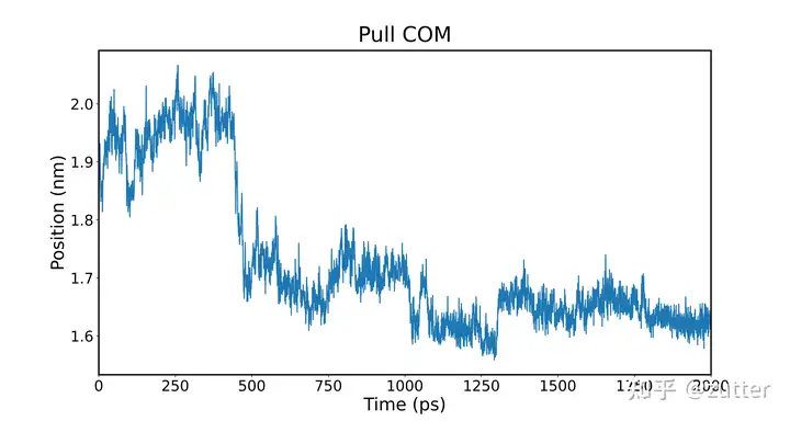
Pullx
查看每个设定DISTANCE的拉伸效果,即查看两个球是否按照我们设定的一样保持一定的距离。
Gromacs在pull模拟时会给出md_pullx.xvg,使用文本工具打开,可以看出我们设置了3个拉伸坐标,因此数据有四列,第一列:模拟时间;第二至四列:每个pull坐标的DISTANCE。
上图可能只想取观察某个坐标的变化,只需要修改plt.plot(df[0], df2)选择想要绘制的数据即可,例:plt.plot(df[0], df[1])
使用简单的python脚本xvg_pullx.py进行绘制
# xvg_pullx.py
1 2 3 4 5 6 7 8 9 10 11 12 13 14 15 16 17 18 19 20 21 22 23 24 25 26 27 28 29 30 31 32 33 34 35 36 import pandas as pdimport numpy as npimport matplotlib.pyplot as pltimport reimport sysdef distance (dat ): with open (dat) as f: lines = f.readlines() labelName = [l for l in lines if l.startswith('@' )] data = [[float (i) for i in l.split()] for l in lines if not ( l.startswith('#' ) or l.startswith('@' ))] title = re.findall(r'\"([\w\d\s\(\)\/]+)\"' , labelName[0 ])[0 ] xlabel = re.findall(r'\"([\w\d\s\(\)\/]+)\"' , labelName[1 ])[0 ] ylabel = re.findall(r'\"([\w\d\s\(\)\/]+)\"' , labelName[2 ])[0 ] df = pd.DataFrame(data) plt.figure(figsize=(15 , 8 )) plt.gca().spines["top" ].set_linewidth(2 ) plt.gca().spines["bottom" ].set_linewidth(2 ) plt.gca().spines["left" ].set_linewidth(2 ) plt.gca().spines["right" ].set_linewidth(2 ) plt.rcParams.update({"font.size" : 24 }) df2 = df.drop([0 ], axis=1 ) plt.plot(df[0 ], df2) plt.xticks(fontsize=20 ) plt.yticks(fontsize=20 ) plt.xlabel(xlabel, fontsize=24 ) plt.ylabel(ylabel, fontsize=24 ) plt.xlim(df[0 ].min (), df[0 ].max ()) plt.title(title, pad=12 ) plt.savefig('{}.png' .format (title),dpi=600 ) if __name__ == '__main__' : distance(sys.argv[1 ])
1 python xvg_pullx.py md_pullx.xvg
只需在相应文件夹执行上述命令即可生成pullx图。
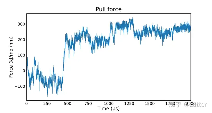
Pullf
pullf的代码与pullx类似,只需将plt.plot(df[0], df[1])更换为plt.plot(df[0],df.drop([0],axis=1))即可。
Position Histrogram
# xvgextract.py
1 2 3 4 5 6 7 8 9 10 11 12 13 14 15 16 17 18 19 20 21 22 23 24 25 26 27 28 29 30 31 32 33 34 35 import pandas as pdimport numpy as npimport matplotlib.pyplot as pltfrom matplotlib.pyplot import MultipleLocatorimport osdef Histogram (): total=pd.DataFrame() plt.figure(figsize=(35 ,8 )) for i in range (28 ): folders=os.getcwd()+"\prod_" +str (i)+"\md_pullx.xvg" with open (folders) as f: lines = f.readlines() labelName=[l for l in lines if l.startswith('@' )] data=[[float (i) for i in l.split()] for l in lines if not (l.startswith('#' ) or l.startswith('@' ))] df=pd.DataFrame(data) total.insert(loc=i,column=i,value=df[1 ]) total[i].hist(stacked=True ,bins=30 ,alpha=0.8 ,histtype="bar" ,edgecolor="black" ) plt.grid(None ) plt.gca().spines["top" ].set_linewidth(2 ) plt.gca().spines["bottom" ].set_linewidth(2 ) plt.gca().spines["left" ].set_linewidth(2 ) plt.gca().spines["right" ].set_linewidth(2 ) plt.rcParams.update({"font.size" :32 }) x_major_locator=MultipleLocator(0.1 ) plt.gca().xaxis.set_major_locator(x_major_locator) plt.xticks(fontsize=24 ) plt.yticks(fontsize=24 ) plt.xlabel("Position (nm)" ,fontsize=32 ) plt.ylabel("Counts" ,fontsize=32 ) plt.title("Position Histogram" ,pad=24 ,fontsize=32 ) plt.savefig('{}.png' .format ("Histogram" ),dpi=600 ) if __name__ == '__main__' : Histogram()
在run文件夹下运行该脚本可以获得如下图片,该图表示采样比较充分,同时在1.8
nm时,两球的排斥力最大,导致了Counts偏下,下面我们着重分析一下在1.8
nm处的相关轨迹。
Histogram
临界值
打开文件夹prod_22(具体哪个文件夹根据自己的模拟情况而定),运行上述分析力和position的代码。
可以看出,在1.8nm左右,因为我们设定的力常数无法限制两个球的位置,导致了突跃。也可以说明在该处两者的吸引力超过了弹簧拉力,C240不能维持原来的位置。
如果弹性常数设定的太大,产生的力会非常小,无法监测到该现象。相应的,当弹性常数过小时,无法将颗粒维持在固定位置。弹性常数可以由下述公式估算\(k=k_b *T /\sigma^2\) 。
总结
本文从建模到构建拓扑到模拟,一步一步地完成了两个胶体分子的模拟。
通过控制两个胶体之间的距离,监测到了临界距离。
因为篇幅有限,所有并没有完成含有离子体系的模拟,但文末提供了阴阳离子的gro和itp文件。
作者水平有限,在行文过程中可能会出现各种各样的问题(包括但不限于原理性、撰写错误等),欢迎指正。
扩展
C24.gro
1 2 3 4 5 6 7 8 9 10 11 12 13 14 15 16 17 18 19 20 21 22 23 24 25 26 27 28 29 30 31 32 33 34 35 36 37 38 39 40 41 42 43 44 45 46 47 48 49 50 51 52 53 54 55 56 57 58 59 60 61 62 63 64 65 66 67 68 69 70 71 72 73 74 75 76 77 78 79 80 81 82 83 84 85 86 87 88 89 90 91 92 93 94 95 96 97 98 99 100 101 102 103 104 105 106 107 108 109 110 111 112 113 114 115 116 117 118 119 120 121 122 123 124 125 126 127 128 129 130 131 132 133 134 135 136 137 138 139 140 141 142 143 144 145 146 147 148 149 150 151 152 153 154 155 156 157 158 159 160 161 162 163 164 165 166 167 168 169 170 171 172 173 174 175 176 177 178 179 180 181 182 183 184 185 186 187 188 189 190 191 192 193 194 195 196 197 198 199 200 201 202 203 204 205 206 207 208 209 210 211 212 213 214 215 216 217 218 219 220 221 222 223 224 225 226 227 228 229 230 231 232 233 234 235 236 237 238 239 240 241 242 243 Great Red Owns Many ACres of Sand 240 1C24 C1 1 0.693 -0.039 0.184 1C24 C2 2 0.690 0.099 0.175 1C24 C3 3 0.644 -0.075 0.309 1C24 C4 4 0.611 0.041 0.377 1C24 C5 5 0.639 0.149 0.294 1C24 C6 6 0.671 0.164 0.054 1C24 C7 7 0.613 0.292 0.060 1C24 C8 8 0.561 0.342 0.181 1C24 C9 9 0.565 0.266 0.299 1C24 C10 10 0.674 0.084 -0.062 1C24 C11 11 0.677 -0.057 -0.052 1C24 C12 12 0.678 -0.121 0.073 1C24 C13 13 0.627 -0.250 0.096 1C24 C14 14 0.577 -0.286 0.223 1C24 C15 15 0.577 -0.194 0.330 1C24 C16 16 0.485 -0.197 0.436 1C24 C17 17 0.451 -0.079 0.505 1C24 C18 18 0.508 0.045 0.469 1C24 C19 19 0.445 0.169 0.488 1C24 C20 20 0.473 0.278 0.404 1C24 C21 21 0.640 0.145 -0.183 1C24 C22 22 0.607 0.281 -0.180 1C24 C23 23 0.580 0.353 -0.062 1C24 C24 24 0.476 0.454 0.179 1C24 C25 25 0.402 0.480 0.296 1C24 C26 26 0.389 0.390 0.403 1C24 C27 27 0.597 -0.328 -0.016 1C24 C28 28 0.621 -0.272 -0.142 1C24 C29 29 0.648 -0.136 -0.164 1C24 C30 30 0.498 -0.401 0.237 1C24 C31 31 0.425 -0.415 0.356 1C24 C32 32 0.406 -0.312 0.450 1C24 C33 33 0.338 -0.076 0.587 1C24 C34 34 0.290 0.050 0.627 1C24 C35 35 0.332 0.172 0.571 1C24 C36 36 0.614 -0.074 -0.287 1C24 C37 37 0.611 0.066 -0.296 1C24 C38 38 0.494 0.465 -0.063 1C24 C39 39 0.443 0.515 0.057 1C24 C40 40 0.246 0.284 0.569 1C24 C41 41 0.274 0.392 0.486 1C24 C42 42 0.292 -0.309 0.533 1C24 C43 43 0.258 -0.192 0.601 1C24 C44 44 0.468 -0.480 0.124 1C24 C45 45 0.517 -0.444 -0.002 1C24 C46 46 0.561 0.337 -0.298 1C24 C47 47 0.531 0.259 -0.409 1C24 C48 48 0.429 0.321 -0.479 1C24 C49 49 0.395 0.437 -0.411 1C24 C50 50 0.477 0.447 -0.299 1C24 C51 51 0.309 0.582 0.288 1C24 C52 52 0.276 0.642 0.168 1C24 C53 53 0.143 0.682 0.175 1C24 C54 54 0.094 0.647 0.299 1C24 C55 55 0.196 0.584 0.369 1C24 C56 56 0.578 -0.345 -0.252 1C24 C57 57 0.545 -0.285 -0.372 1C24 C58 58 0.446 -0.361 -0.433 1C24 C59 59 0.418 -0.468 -0.350 1C24 C60 60 0.499 -0.458 -0.238 1C24 C61 61 0.336 -0.521 0.363 1C24 C62 62 0.307 -0.599 0.252 1C24 C63 63 0.176 -0.644 0.265 1C24 C64 64 0.125 -0.595 0.384 1C24 C65 65 0.224 -0.518 0.444 1C24 C66 66 0.170 0.052 0.697 1C24 C67 67 0.091 -0.062 0.710 1C24 C68 68 -0.041 -0.022 0.717 1C24 C69 69 -0.045 0.116 0.708 1C24 C70 70 0.086 0.162 0.695 1C24 C71 71 0.364 -0.575 0.128 1C24 C72 72 0.194 -0.409 0.524 1C24 C73 73 0.459 -0.505 -0.114 1C24 C74 74 0.553 -0.147 -0.390 1C24 C75 75 0.546 0.121 -0.408 1C24 C76 76 0.434 0.508 -0.183 1C24 C77 77 0.335 0.605 0.048 1C24 C78 78 0.171 0.486 0.463 1C24 C79 79 0.117 0.277 0.624 1C24 C80 80 0.128 -0.184 0.655 1C24 C81 81 0.096 -0.668 0.155 1C24 C82 82 0.158 -0.662 0.029 1C24 C83 83 0.291 -0.616 0.016 1C24 C84 84 -0.009 -0.566 0.399 1C24 C85 85 -0.042 -0.468 0.494 1C24 C86 86 0.058 -0.390 0.556 1C24 C87 87 -0.043 -0.658 0.175 1C24 C88 88 -0.095 -0.607 0.296 1C24 C89 89 0.340 -0.580 -0.110 1C24 C90 90 0.258 -0.590 -0.224 1C24 C91 91 0.292 -0.525 -0.344 1C24 C92 92 0.199 -0.482 -0.440 1C24 C93 93 0.227 -0.372 -0.524 1C24 C94 94 0.350 -0.304 -0.514 1C24 C95 95 0.368 -0.169 -0.549 1C24 C96 96 0.468 -0.091 -0.487 1C24 C97 97 0.465 0.048 -0.496 1C24 C98 98 0.361 0.112 -0.568 1C24 C99 99 0.336 0.249 -0.552 1C24 C100 100 0.210 0.309 -0.570 1C24 C101 101 0.176 0.427 -0.501 1C24 C102 102 0.266 0.488 -0.413 1C24 C103 103 0.228 0.567 -0.303 1C24 C104 104 0.311 0.576 -0.189 1C24 C105 105 0.260 0.627 -0.069 1C24 C106 106 0.125 0.668 -0.062 1C24 C107 107 0.062 0.687 0.063 1C24 C108 108 -0.076 0.672 0.084 1C24 C109 109 -0.126 0.636 0.211 1C24 C110 110 -0.039 0.613 0.319 1C24 C111 111 0.037 0.464 0.498 1C24 C112 112 -0.067 0.527 0.427 1C24 C113 113 0.024 -0.273 0.625 1C24 C114 114 -0.111 -0.232 0.632 1C24 C115 115 -0.144 -0.101 0.670 1C24 C116 116 0.009 0.356 0.582 1C24 C117 117 -0.124 0.309 0.595 1C24 C118 118 -0.151 0.183 0.651 1C24 C119 119 -0.261 -0.035 0.629 1C24 C120 120 -0.265 0.106 0.619 1C24 C121 121 -0.644 0.075 -0.309 1C24 C122 122 -0.611 -0.041 -0.376 1C24 C123 123 -0.693 0.039 -0.184 1C24 C124 124 -0.690 -0.099 -0.175 1C24 C125 125 -0.639 -0.149 -0.294 1C24 C126 126 -0.508 -0.045 -0.469 1C24 C127 127 -0.445 -0.169 -0.488 1C24 C128 128 -0.473 -0.278 -0.404 1C24 C129 129 -0.565 -0.266 -0.298 1C24 C130 130 -0.451 0.079 -0.505 1C24 C131 131 -0.485 0.197 -0.436 1C24 C132 132 -0.577 0.194 -0.330 1C24 C133 133 -0.577 0.286 -0.223 1C24 C134 134 -0.627 0.250 -0.096 1C24 C135 135 -0.678 0.121 -0.073 1C24 C136 136 -0.677 0.057 0.052 1C24 C137 137 -0.674 -0.084 0.062 1C24 C138 138 -0.671 -0.164 -0.054 1C24 C139 139 -0.613 -0.292 -0.059 1C24 C140 140 -0.561 -0.342 -0.181 1C24 C141 141 -0.338 0.076 -0.587 1C24 C142 142 -0.290 -0.050 -0.627 1C24 C143 143 -0.332 -0.172 -0.571 1C24 C144 144 -0.389 -0.390 -0.402 1C24 C145 145 -0.402 -0.480 -0.296 1C24 C146 146 -0.476 -0.454 -0.179 1C24 C147 147 -0.498 0.401 -0.237 1C24 C148 148 -0.425 0.415 -0.356 1C24 C149 149 -0.406 0.312 -0.450 1C24 C150 150 -0.597 0.328 0.016 1C24 C151 151 -0.621 0.272 0.142 1C24 C152 152 -0.648 0.136 0.164 1C24 C153 153 -0.641 -0.145 0.183 1C24 C154 154 -0.607 -0.281 0.180 1C24 C155 155 -0.580 -0.353 0.062 1C24 C156 156 -0.292 0.309 -0.533 1C24 C157 157 -0.258 0.192 -0.601 1C24 C158 158 -0.246 -0.284 -0.569 1C24 C159 159 -0.274 -0.392 -0.485 1C24 C160 160 -0.495 -0.465 0.063 1C24 C161 161 -0.443 -0.515 -0.057 1C24 C162 162 -0.614 0.074 0.287 1C24 C163 163 -0.611 -0.066 0.296 1C24 C164 164 -0.517 0.444 0.002 1C24 C165 165 -0.468 0.480 -0.124 1C24 C166 166 -0.170 -0.052 -0.696 1C24 C167 167 -0.092 0.062 -0.710 1C24 C168 168 0.041 0.022 -0.717 1C24 C169 169 0.044 -0.116 -0.708 1C24 C170 170 -0.086 -0.162 -0.695 1C24 C171 171 -0.309 -0.582 -0.288 1C24 C172 172 -0.196 -0.584 -0.369 1C24 C173 173 -0.094 -0.647 -0.299 1C24 C174 174 -0.143 -0.682 -0.175 1C24 C175 175 -0.276 -0.642 -0.168 1C24 C176 176 -0.336 0.521 -0.363 1C24 C177 177 -0.224 0.518 -0.444 1C24 C178 178 -0.125 0.595 -0.384 1C24 C179 179 -0.177 0.644 -0.265 1C24 C180 180 -0.307 0.599 -0.252 1C24 C181 181 -0.578 0.345 0.252 1C24 C182 182 -0.499 0.458 0.238 1C24 C183 183 -0.418 0.468 0.350 1C24 C184 184 -0.446 0.361 0.433 1C24 C185 185 -0.545 0.284 0.372 1C24 C186 186 -0.561 -0.337 0.298 1C24 C187 187 -0.531 -0.259 0.409 1C24 C188 188 -0.429 -0.321 0.479 1C24 C189 189 -0.395 -0.437 0.411 1C24 C190 190 -0.477 -0.447 0.300 1C24 C191 191 -0.459 0.505 0.114 1C24 C192 192 -0.553 0.147 0.390 1C24 C193 193 -0.364 0.575 -0.128 1C24 C194 194 -0.194 0.409 -0.524 1C24 C195 195 -0.128 0.184 -0.655 1C24 C196 196 -0.117 -0.277 -0.624 1C24 C197 197 -0.172 -0.486 -0.463 1C24 C198 198 -0.335 -0.605 -0.048 1C24 C199 199 -0.434 -0.508 0.183 1C24 C200 200 -0.546 -0.121 0.408 1C24 C201 201 -0.292 0.525 0.344 1C24 C202 202 -0.258 0.590 0.224 1C24 C203 203 -0.341 0.580 0.110 1C24 C204 204 -0.350 0.304 0.514 1C24 C205 205 -0.368 0.169 0.549 1C24 C206 206 -0.468 0.091 0.487 1C24 C207 207 -0.199 0.482 0.440 1C24 C208 208 -0.227 0.372 0.524 1C24 C209 209 -0.291 0.616 -0.016 1C24 C210 210 -0.158 0.662 -0.029 1C24 C211 211 -0.096 0.668 -0.155 1C24 C212 212 0.043 0.658 -0.174 1C24 C213 213 0.095 0.607 -0.296 1C24 C214 214 0.009 0.566 -0.399 1C24 C215 215 0.042 0.468 -0.494 1C24 C216 216 -0.059 0.390 -0.556 1C24 C217 217 -0.024 0.273 -0.624 1C24 C218 218 0.111 0.232 -0.632 1C24 C219 219 0.144 0.101 -0.670 1C24 C220 220 0.261 0.035 -0.629 1C24 C221 221 0.265 -0.106 -0.619 1C24 C222 222 0.151 -0.183 -0.651 1C24 C223 223 0.124 -0.309 -0.595 1C24 C224 224 -0.009 -0.356 -0.582 1C24 C225 225 -0.037 -0.464 -0.498 1C24 C226 226 0.067 -0.528 -0.427 1C24 C227 227 0.039 -0.613 -0.319 1C24 C228 228 0.126 -0.636 -0.211 1C24 C229 229 0.076 -0.672 -0.084 1C24 C230 230 -0.062 -0.687 -0.063 1C24 C231 231 -0.260 -0.627 0.069 1C24 C232 232 -0.125 -0.668 0.062 1C24 C233 233 -0.465 -0.048 0.496 1C24 C234 234 -0.361 -0.112 0.568 1C24 C235 235 -0.336 -0.249 0.552 1C24 C236 236 -0.312 -0.577 0.189 1C24 C237 237 -0.229 -0.567 0.303 1C24 C238 238 -0.267 -0.488 0.413 1C24 C239 239 -0.210 -0.309 0.571 1C24 C240 240 -0.176 -0.427 0.502 0.00000 0.00000 0.00000
构建NH4+原子gro
原子结构文件可以使用pubchem查找下载,也可以使用绘图工具绘制之后,使用gaussian/orca优化之后,使用Sobtop
(sobereva.com) 构建分子top,如果使用sobtop,需要注意将atomtypes提取到总topol开头处。此处使用教程中提供的文件。
# NH4.gro
1 2 3 4 5 6 7 8 9 NH4 5 1NH4 N 1 0.000 -0.000 0.000 1NH4 H1 2 0.091 0.037 -0.035 1NH4 H2 3 -0.014 -0.097 -0.035 1NH4 H3 4 -0.078 0.061 -0.035 1NH4 H4 5 0.000 -0.000 0.104 0.00000 0.00000 0.00000
# NH4.itp
1 2 3 4 5 6 7 8 9 10 11 12 13 14 15 16 17 18 19 20 21 22 23 24 25 26 27 28 [ moleculetype ] ; name nrexcl NH4 3 [ atoms ] ; nr type resnr residu atom cgnr charge mass 1 opls_ 286 1 NH4 N 1 2 opls_ 289 1 NH4 H1 1 3 opls_ 289 1 NH4 H2 1 4 opls_ 289 1 NH4 H3 1 5 opls_ 289 1 NH4 H4 1 [ bonds ] ;ai aj funct 1 2 1 1 3 1 1 4 1 1 5 1 [ angles ] ;ai aj ak funct 2 1 3 1 2 1 4 1 2 1 5 1 3 1 4 1 3 1 5 1 4 1 5 1
构建NO3-原子gro
# NO3.gro
1 2 3 4 5 6 7 8 NO3 4 1NO3 N 1 -0.008 -0.022 0.010 1NO3 O1 2 -0.043 -0.015 -0.085 1NO3 O2 3 -0.043 0.058 0.064 1NO3 O3 4 0.094 -0.022 0.010 0.00000 0.00000 0.00000
# NO3.itp
1 2 3 4 5 6 7 8 9 10 11 12 13 14 15 16 17 18 19 20 21 22 23 24 25 26 27 [ moleculetype ] ; name nrexcl NO3 3 [ atoms ] ; nr type resnr residu atom cgnr charge mass 1 opls_ 787 1 NO3 N 1 2 opls_ 788 1 NO3 O1 1 3 opls_ 788 1 NO3 O2 1 4 opls_ 788 1 NO3 O3 1 [ bonds ] ;ai aj funct 1 2 1 1 3 1 1 4 1 [ angles ] ; ai aj ak funct 2 1 3 1 2 1 4 1 3 1 4 1 ; [ dihedrals ] ;ai ai ak al funct 2 1 3 4 2