Electronic Circular Dichroism

计算圆二色谱ECD

Electronic Circular Dichroism

电子圆二色谱


Electronic Circular Dichroism(ECD)是一种与紫外可见光谱相关的方法,利用圆形偏振光而不是常规的非偏振光,有助于鉴定手性化合物

作为例子,假设,你需要判断某些物质的纯度。该物质具有+/-异构体,并且没有其他结构。
../_images/cod_struct.png

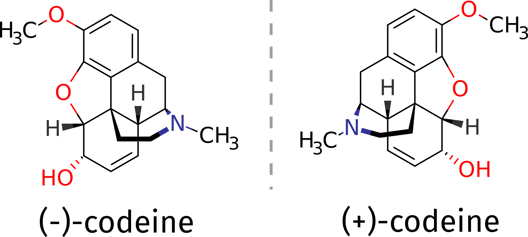
(-)异构体用于医疗领域,可以使用ORCA计算纯化合物的ECD光谱,借助理论来区分异构体

Predicting ECD spectra

使用TD-DFT预测物质在水中的圆二色谱。

The mains steps to obtain the ECD spectra from TD-DFT are the same as those for UV/Vis. Please read the related UVVis spectroscopy section before going any further. From now on that will be assumed as known.

第一步是绘制并优化此分子的几何构型

1
2
!B3LYP DEF2-TZVP D4 OPT FREQ CPCM(WATER)
* XYZfile 1 1 minuscodeine_guess.xyz

电荷数为+1,因为我们希望在水中再现此物质的碱性圆二色谱,pKa为8。
使用TD-DFT方法时,ECD光谱被自动计算,输入如下

1
2
3
4
5
!B3LYP DEF2-TZVP CPCM(WATER)
%TDDFT
NROOTS 25
END
* XYZfile 1 1 codeine_optimized.xyz

考虑水对电子结构的影响,对于基态使用CPCM模型。对于激发态使用LR-CPCM模型(!CPCM自动选择)

极性溶剂对带电分子的激发态有很大影响,不忘记考虑这些因素

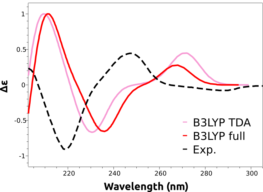
因为ECD对于转换的预测强度特别敏感,我们需要使用完整的TD-DFT计算而不是使用TDA近似。
通常,TDA“能够提供更稳定更可靠的结果,但使用TD-DFT时,ECD预测结果更好,输入为:

1
2
3
4
5
6
!B3LYP DEF2-TZVP CPCM(WATER)
%TDDFT
NROOTS 25
TDA FALSE
END
* XYZfile 1 1 codeine_optimized.xyz

使用TDA FALSE来限制使用TDA近似

1
2
3
4
5
6
7
8
9
10
11
12
# ECD光谱
-------------------------------------------------------------------
CD SPECTRUM
-------------------------------------------------------------------
State Energy Wavelength R MX MY MZ
(cm-1) (nm) (1e40*cgs) (au) (au) (au)
-------------------------------------------------------------------
1 38539.1 259.5 -7.97318 -0.08936 -0.09057 0.28910
2 39977.7 250.1 32.07887 0.18900 -0.02049 -0.22614
3 43324.1 230.8 12.30861 -0.09352 -0.02155 0.30521
4 44246.4 226.0 -85.09304 0.38524 0.23404 -0.59099
5 46657.1 214.3 50.33474 0.08844 -0.07182 0.09990

在能量之后紧跟着是激发波长,激发波长的R值(与ECD强度成比例),磁性偶极子组成
更加详细的描述可以从激发态分析中获得

Shifting the predicted spectra

使用Avogadro打开.out文件,绘制谱图
../_images/b3lyp.png

计算光谱右移,在预测过程中很常见,这是由于计算激发态能量引起的预期误差。这些误差相当系统,能够通过对预测进行反转来消除
../_images/b3lyp_shifted.png

The shift is not given in nanometers, but in energy units, because the wavelength is not directly proportional to the energy. However common in the literature, there is not much sense to apply a shift in wavelength scale, since the energy correction would be different for each peak!

Comparing functionals

仔细看看预测的光谱将揭示他们缺乏负能带,这对应于(-)立体异构体。这是由B3LYP函数引起的错误,无法预先知道
我们可以使用更高级别的无参数化方法DLPNO-STEOM,或者不同的功能函数。
range-separated functionals对于此案例适用,我们可以使用 wB97x函数进行计算

1
2
3
4
5
!wB97X DEF2-TZVP CPCM(WATER)
%TDDFT
NROOTS 25
END
* XYZfile 1 1 codeine_optimized.xyz
../_images/wb_shifted.png

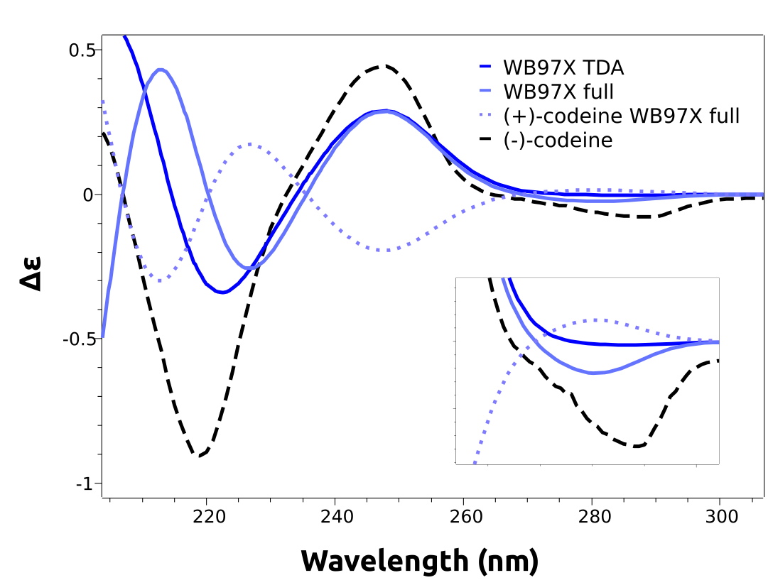
使用此方法,可以预测低能带。甚至可以绘制其他立体异构体的计算频谱。

There is no need to reoptimize the geometry when looking for stereoisomers. These can be easily generated by choosing one axis, e.g the z, and multiplying all components of the coordinates along that by -1. That is equivalent to a reflection over the xy plane, which generates the “mirror image” of our target molecule.

ECD spectra are very sensitive to minor geometrical changes! Usually we can only get results close to the experiment by computing the lower energy conformers and making a Boltzmann sum. In this case, the molecule is rather rigid and the problem was minimized, however that is not the usual case.

Structure

1
2
3
4
5
6
7
8
9
10
11
12
13
14
15
16
17
18
19
20
21
22
23
24
25
26
27
28
29
30
31
32
33
34
35
36
37
38
39
40
41
42
43
44
C          0.27861       -2.51771       -1.18929
C 1.62027 -2.60915 -0.76912
C 2.22334 -1.60792 0.00987
O 3.54007 -1.82025 0.28510
C 1.43672 -0.52943 0.36578
O 1.82325 0.61959 1.00916
C 0.09858 -0.48519 0.01418
C -0.55354 0.74611 0.55554
C 0.72840 1.57467 0.78794
C 1.08903 2.56775 -0.35541
O 2.47118 2.53561 -0.68410
C 0.30918 2.41405 -1.62915
C -0.90175 1.83953 -1.69766
C -1.56787 1.27202 -0.47255
C -2.56293 0.10674 -0.76050
N -3.31366 -0.16885 0.56397
C -4.50113 -1.08483 0.41229
C -2.41884 -0.59039 1.70688
C -1.27044 0.40261 1.87918
C -1.88442 -1.17437 -1.33429
C -0.50047 -1.42947 -0.80310
C 4.17091 -0.93416 1.20079
H -0.12034 -3.29174 -1.84231
H 2.21941 -3.46198 -1.08750
H 0.64670 2.15619 1.71529
H 0.88257 3.58363 0.00417
H 2.81653 1.66581 -0.40960
H 0.75014 2.85301 -2.52332
H -1.42425 1.82856 -2.65248
H -2.13625 2.10396 -0.03138
H -3.34042 0.44534 -1.45658
H -5.10054 -0.72966 -0.42961
H -5.08559 -1.02485 1.33453
H -4.15126 -2.10599 0.24932
H -2.06881 -1.60774 1.50636
H -3.03858 -0.61066 2.61016
H -1.66742 1.32913 2.31529
H -0.56791 -0.00565 2.61746
H -2.50583 -2.06189 -1.18461
H -1.78792 -1.03545 -2.41928
H 5.17371 -1.32388 1.40176
H 3.63531 -0.89593 2.15499
H 4.28807 0.06211 0.76383
H -3.72689 0.73229 0.84204