预测EPR特性和光谱
Predicting EPR
使用ORCA预测EPR特性和光谱,其中甚至包括许多复杂的问题(自旋轨道耦合和其他相对论效应)
The CH3 radical
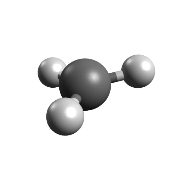
甲基自由基
甲基自由基是一种平面分子,其平面性部分已被EPR光谱证实。
It has a g of 2.0025 and hyperfine couplings (HFC) Axx=−31.4,Ayy=−93.7, and Azz=−60.30,let’s try to predict that from first principles!
优化结构
1 | !B3LYP DEF2-TZVP OPT |
你将得到优化后的三角平面坐标
下一步是计算EPR性质,通过设置%EPRNMP计算。
重点:这些是ORCA输入的唯一选项,应该几何优化之后
An input to compute the g tensor and HFCs for the hydrogen atoms, using the B3LYP functional could be:
1 | !B3LYP EPR-II AUTOAUX |
- The
GTENSORflag must be set to TRUE in order to compute it, the default is FALSE.- The
NUCLEIdefines the atoms for the HFC calculation.ALL Hcalculates the HFC on all hydrogens, or useALL N,ALL Cand so on for different atoms. You can also useNUCLEI = 1,5,8, to give one list per atom type with the atom numbering staring from 1.- The
AISO,ADIPandAORBflags request the isotropic part of the HFC, its dipolar part and 2nd order contribution from SOC respectively.- The
AORBterm is costly, but contributes very little to organic molecules without heavy atoms and could be neglected in those cases.- A large basis is recommended for EPR properties. Here we used the special basis EPR-II, for more info one can check the full documentation.
- The spin-orbit coupling integrals are calculated using the
SOMF(1X)method by default, but more efficient options are also available.
If you are using a list of atoms, like NUCLEI = 1,5,8, there should be one list for each atom type!
The output file
在单点能计算成功后,第一步是计算用于处理SOC的积分
1 | ------------------------------------------------------------------------------ |
1 | ------------------------------------------------------------------------------ |
Please notice that the “Origin for angular momentum” here is “Center of electronic charge”, and that means these results are not gauge-invariant and can change depending on your coordinates.
The calculation of the integrals involving GIAOs is much more costly than the regular ones, so be prepared for longer calculation times.
Usually, with a sufficiently large basis, the results should be almost invariant, but if one wants the exact results, gauge-invariant atomic orbitals (GIAOs) are needed . These can be constructed from all basis sets, and to use them, just add ORI GIAO to the %EPRNMR section:
1 | %EPRNMR |
g Tensor
If the following CP-SCF converges, you will get the g tensor matrix:
1 | ------------------- |
Here the components of the g tensor are specified and the total components for the x, y and z directions are printed after g(tot), with the isotropic value afterwards. The Delta-g shown is the difference from the free-electron g value.
As you can see, the predicted value is already quite close to the experimental value, considering we completely ignored any matrix effects and its largest deviation from the free-electron comes due to SOC effects, as suggested by Gordy.
Hyperfine couplings
After the g tensor calculation, comes the HFC for each atom:
1 | ----------------------------------------- |
Here “I=” indicates the spin of that given atom and “P=” is the proportionality factor μeμNβeβNμeμNβeβN used. After that, another CP-SCF solution is requested and the HFC information is printed:
1 | Raw HFC matrix (all values in MHz): |
Again, the individual components are printed and the A(iso) is shown in the end. As you can see, the results are in quite good agreement with the experimental data.
At the very end, the ORCA EULER output is printed, with information about the relative angle between the g-tensor and the HFCs, which have an arbitrary relationship from the calculation:
1 | ------------------------------------------------------------------------- |
You can use the orca_euler software later if you want to rotate any of these for any specific application.
Comparison to experiment
To summarize our results, here is a table comparing the calculated and predicted data:
With these, one can use tools such as EasySpin, which already has a specific function for reading orca outputs and simulate the EPR spectrum. The comparison between the theory prediction and an EPR spectra taken at 4K in a CH4 matrix is:


Of course differences here are expected due to impurities and matrices effects and the graphic was displaced to match the gg.
The HFCs are quite sensitive to the geometry of the molecules! Be sure to have a good one before computing them.
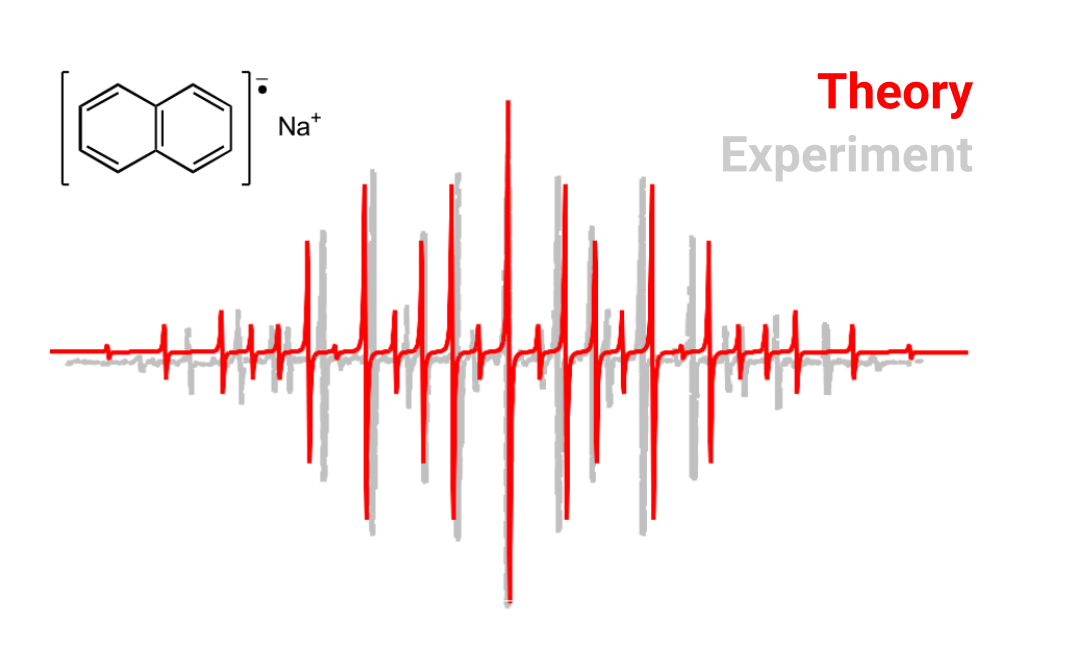
Another example, the naphthalene anion radical
In aprotic solvents and in the presence of alkali metals, polyaromatics such as naphthalene can reduce to form radical anions
These will present nice EPR spectra, with two sets of four protons and thus more complex lines. To predict its spectrum, again one can start by optimizing the geometry of the anion:
1 | !RI-B2PLYP DEF2-TZVP DEF2-TZVP/C TIGHTOPT |
We used a double-hybrid functional to add RI-MP2 correlation and get a better density and TIGHTOPT to obtain a good symmetrical geometry.
Now we run an EPR calculation, with the specialized EPR-III basis and RI-SOMF(1X) to speed-up the calculation of the integrals for the SOC part:
1 | !RI-B2PLYP EPR-III AUTOAUX RI-SOMF(1X) |
One can average the two sets of similar HαHα and HβHβ couplings (calculated from the MP2 relaxed density ) and use again some software like EasySpin to compute the predicted spectrum and compare it to the experiment. This will look like:
Visualizing the g tensor orientation
You can use Avogadro to visualize the orientation of the g tensor. Here is how it works: ORCA prints a basename.gori.xyz file, where dummy atoms are used to represent these vectors, He for the origin, Ne for the direction of gz, Ar for gy and Kr for gx
- Open this file and select the “Align” option in Avogadro, on the right of the “E” used for optimization.
- Now select the He-Ne bond and align the x axis and repeat in order for the y and z axis.
- Delete the noble gas atoms.
- Click on “Axes”, the first option of the “Display Settings”. Here it is!
You can increase the size of the vectors by clicking on the “Axes” options. The order is red for x, green for y and blue for z (remember the RGB sequence).
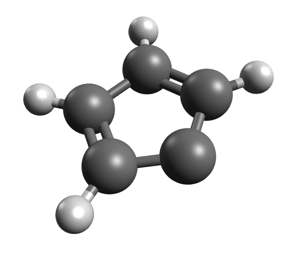
Zero-field Splitting (ZFS)
If you have systems with S>1/2, you might be interested in ZFS values. The ORCA_EPRNMR module can also be used to predict those. Let’s try the example of cyclopentadienylidene carbene, which has known D value of 0.408cm−1 and a E/Dratio of 0.046 . First, the geometry is optimized using:
1 | !B3LYP DEF2-TZVP OPT |
The ZFS can then be computed on simple DFT level using:
1 | !B3LYP EPR-II AUTOAUX UNO |
The DTENSOR flag asks to include the spin-spin and the spin-orbit components of the D (SSANDSO), and the DSS and DSOC control the specific algorithms. For more information, consult the ORCA manual.
After the calculation of the SOC-related integrals, one should see the header:
1 | ------------------------------------------------------------------------------ |
explaining the details of the calculation. The actual result is below the CP-SCF:
1 | D = 0.425943 cm**-1 |
which is again close to the experiment, considering that we are using DFT and a single-reference method.
This was intended to be a simple demonstration. In general, much better results for ZFS can be obtained from multi-reference theories such as CASSCF or MRCI. Nonetheless, it is still quite good and is easily applicable to large systems.
Structures
1 | # Napthalene |