预测紫外可见光谱
预测电子激发态、能量
UVVis spectroscopy
紫外可见分光光度计
预测紫外/可见光谱,对于预测系统的电子激发态、能量以及跃迁概率十分重要
在ORCA中,有多种方法以不同精度预测激发态性质。
在这,只讨论两种:
最简单和广泛使用的TD-DFT,在精度和速度之间有一个很好的权衡
新方法STEOM-DLPNO-CCSD,计算激发态更加准确
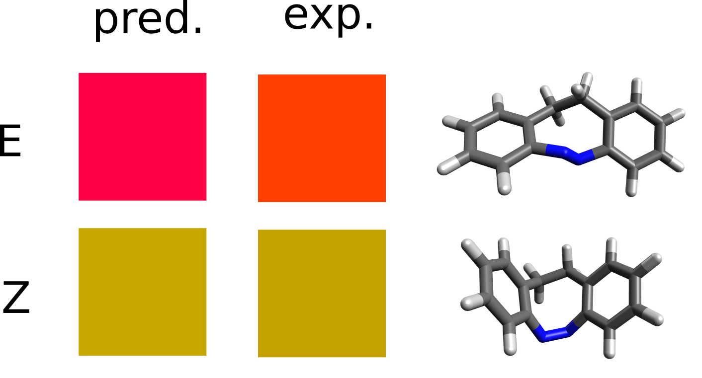
Case study - azobenzene E/Z isomers
案例:偶氮苯E/Z异构体
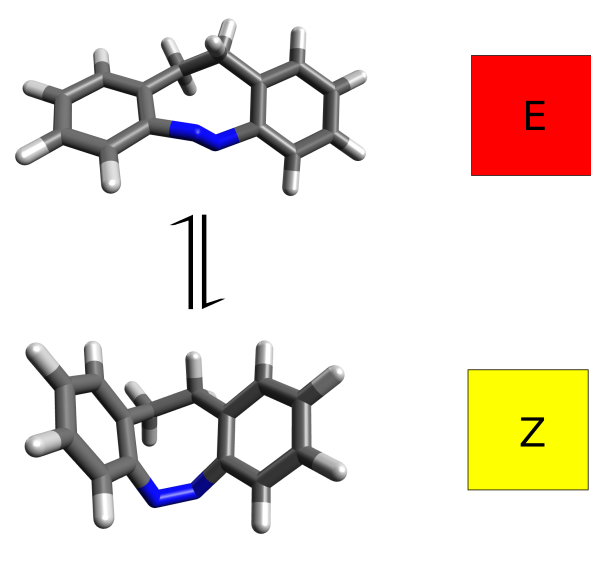
It turns out that the E and Z isomers have different colors - one is yellow and the other red - and the authors attribute this to a change in the lower energy band, assigned as a n−π∗ transition. Let’s see how we could have predicted these results from first principles.
TD-DFT
瞬态密度泛函理论(time-dependent density functional theory (TD-DFT) )是最常用用于预测紫外/可见光谱的方法,简单且廉价2.
ORCA使用,B3LYP 三重态基组
1 | !B3LYP DEF2-TZVP CPCM(HEXANE) |
%TDDFT自动请求光谱预测所需的激发态计算,NROOTS设置要控制的激发态数量
Here we also used the CPCM as a solvation model for both the ground and the excited states to simulate the hexane used in the experiment, which for the excited state case means the LR-CPCM model by default. After the regular SCF, the TD-DFT header is printed:
1 | ------------------------------------------------------------------------------ |
ORCA中TD-DFT默认使用TDA近似,可以通过设置%TDDFT TDA FALSE关闭
1 | # 构建积分网格 |
Note that the RI and COSX approximations are also used to compute the necessary integrals for the TD-DFT solution. The error here is usually even smaller than in the SCF, and the calculation runs much faster (by a factor of about 10), so it is highly recommended to use these.
Printing of the excited states
1 | # 输出收敛态 |
It is important to have in mind that these energies actually are the vertical energy differences, or the energy of that state in the ground state geometry.
Below the energies, the contributions of each single excitation are printed, first with its relative contribution (these will be discussed later), followed by the eigenvector value.
The electronic spectrum
在CPCM校正后,ORCA会计算一些必要的积分
1 | ----------------------------- |
输出光谱
1 | ----------------------------------------------------------------------------- |
The states and their respective vertical transition energies are printed again, now together with the oscillator strength and transition dipole moments. Strictly speaking, this is yet not a “spectrum” like the experimental one because we only have transition lines, not bands.
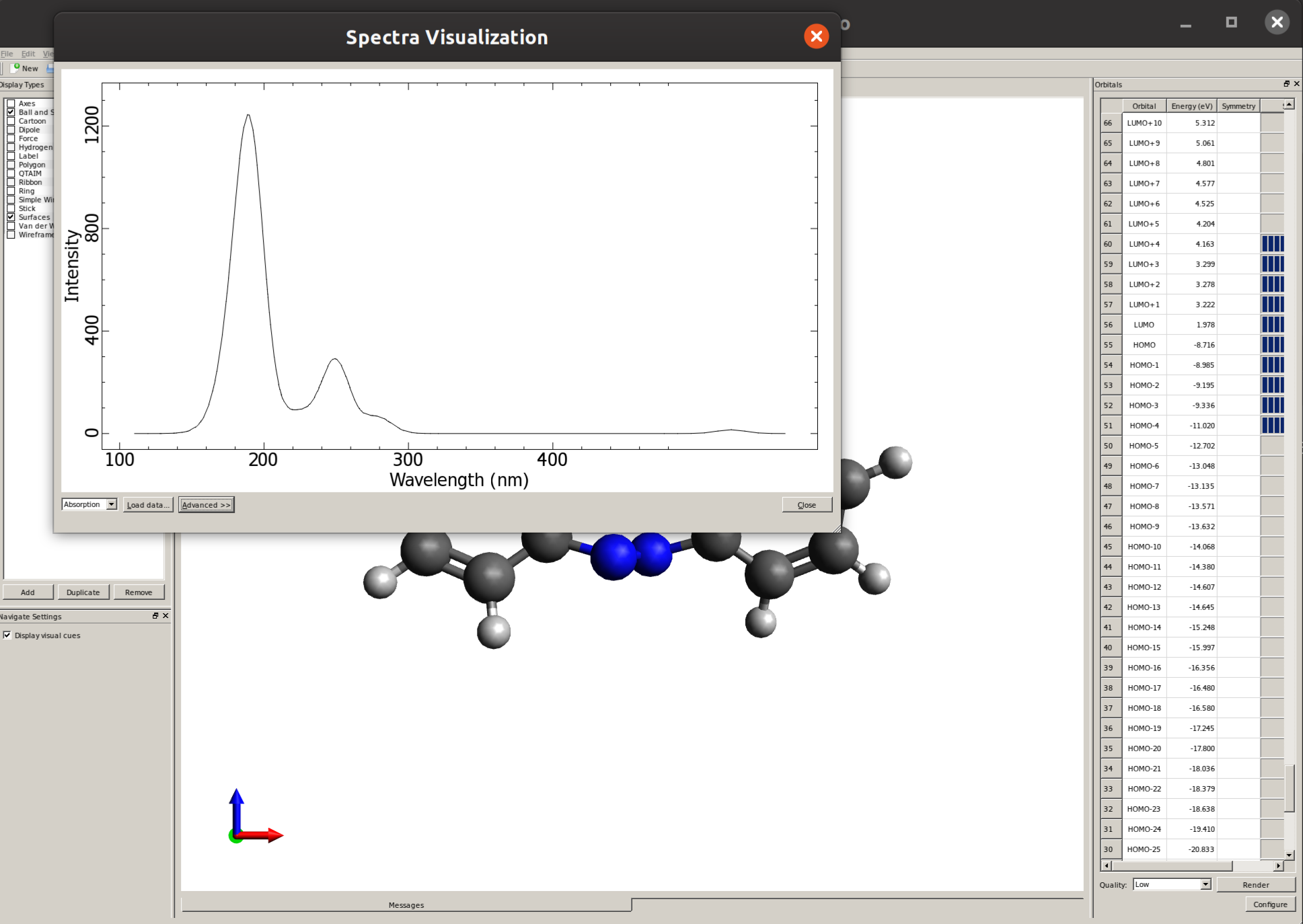
Plotting the calculated spectrum
What we can do to approximate the experimental spectrum then is, e.g, convolute these lines with a Gaussian function to turn them into bands. This can be done easily by using Avogadro: open the output file, then go into ``“Extensions”
and then“Spectra…”to open the“Spectra Visualization”` window:
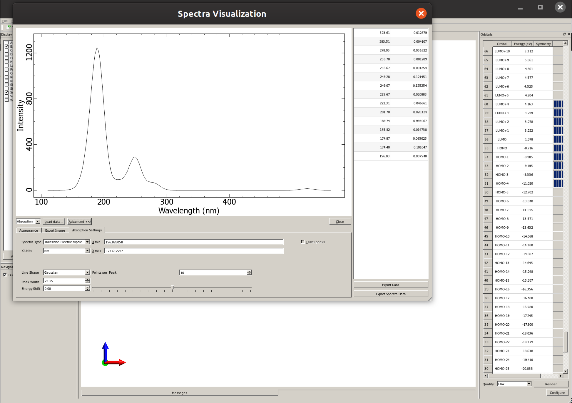
There you can click on
"Advanced"and then"Absorption Settings"to set the details such as the line width and even"Export Spectra Data"to replot this graphic using a different software:
Back to the example
Here is a plot of the predicted spectrum for both the E and Z isomers obtained from the calculation above, using B3LYP and the DEF2-TZVP basis:
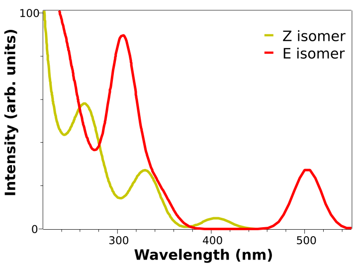
The two low energy peaks at about 507 and 417 nm for the E and Z isomers match quite well the experimental results of 490 and 404 nm. If one converts this wavelength to color and takes its complementary, the correspondence is fairly good:
It is not that common that these results agree so well to the experiment, and here it can be somewhat accidental. It is much more prevalent that the predicted spectra is “shifted” by ±0.1 to ±0.5 eV and it is costumary in the literature to fix that, if there is any reference, to correct systematic errors.
Analysis of the excited states
激发态分析
偶氮苯中光谱带的分配:低能量峰对应S1状态,即具有n−π∗特征,较高能量峰对应S2状态,即具有 π−π∗状态,对异构化过程具有重要影响
通过检查激发态组成,我们可以利用计算结果来帮助完成这项复杂的任务。TD-DFT输出得第一激发态组成如下所示
1 | STATE 1: E= 0.089757 au 2.442 eV 19699.5 cm**-1 <S**2> = 0.000000 |
S1状态有94%概率从54轨道到轨道55,HOMO到LUM的跃迁组成(a表示alpha轨道)
如果使用关键词!LARGEPRINT,能够打开basename.out文件查看轨道

HOMO是n-like分子轨道,主要位于氮的孤立电子对上,LUMO是π∗轨道,主要围绕N=N键
也输出了S2主要组成,94% HOMO-1到LUMO的转变。从上图可以看出HOMO-1更像常规的π 轨道
Avogadro counts orbitals starting from 1, but ORCA starts counting from 0. So orbital 54 in ORCA will be orbital 55 in Avogadro, and so on!
Natural transition orbitals (NTOs)
自然过渡轨道
研究激发态性质的另一种方法就是查看每个跃迁的NTO
1 | STATE 13: E= 0.213089 au 5.798 eV 46767.6 cm**-1 <S**2> = 0.000000 |
至少包含七个大的过渡,如果使用DONTO TRUE计算TD-DFT
1 | !B3LYP DEF2-TZVP CPCM(HEXANE) |
激发态的NTO会被打印
1 | ------------------------------------------ |
the S13 is now described in terms of only two main transitions. These NTOs are saved in a file named basename.s13.nto, and can be printed using the orca_plot tool.
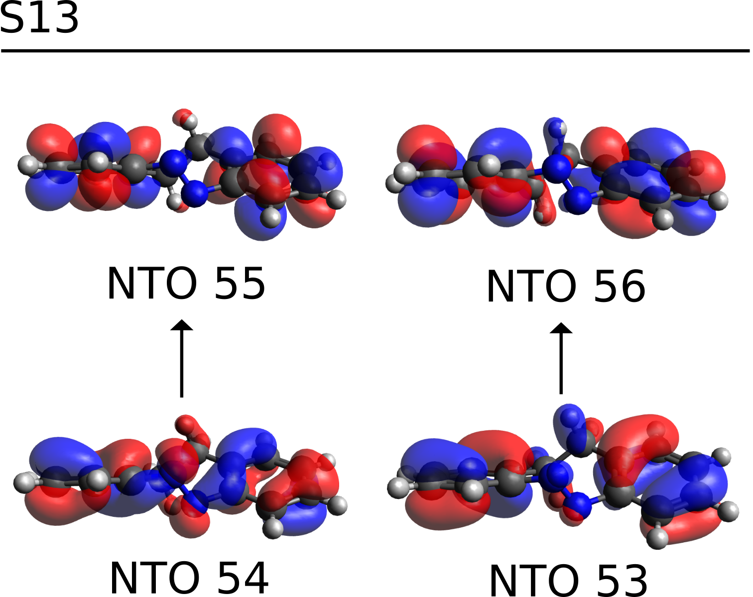
which are clearly π−π∗ transitions on the aromatic rings, and S13S13 can then be assigned as such
A higher level method - STEOM-DLPNO-CCSD
高等级计算方法 STEOM-DLPNO-CCSD
As shown above, TD-DFT can be successful in many cases when trying to predict excited states, however one can not know a priori if a given functional will work or not and different functionals are bound to give different results.
In order to avoid this trial-and-error between functionals, an ab initio unparametrized method is sometimes a better choice. In ORCA, many of these methods are available, but for the sake of simplicity we will show here one that has a very good accuracy, still at an affordable computational cost: the Similarity Transformed Equation of Motion CCSD (STEOM-CCSD).
The STEOM-CCSD is a method that also includes Correlation energy into the calculation of the excited states, thus increasing the quality of the prediction [Iszak2019a]. It is in itself a heavy method and very computational demanding, but the ORCA team has recently developed The DLPNO scheme version of it (DLPNO-STEOM), that presents a much better scaling and it is not much costlier than TD-DFT [Iszak2019b].
In order to use that, just optimize your geometry somehow and run:
1 | !STEOM-DLPNO-CCSD DEF2-TZVP DEF2-TZVP/C RIJCOSX CPCM(HEXANE) |
As in other DLPNO or correlated methods using the RI, the /C basis is necessary for the calculation. We also added the CPCM correction for both the ground and excited states, here the latter is invoked by setting DOSOLV TRUE under %MDCI, which is the block that controls these calcualtions.
The MAXITER 100 defines the maximum number of iterations during the many steps of STEOM, and sometimes it is necessary to increase it to achieve convergence.
The output printed is much larger than that of TD-DFT, for there are many more steps necessary to conclude the overall computation. In summary what is done is:
- First a regular DLPNO-CCSD calculation is performed.
- That is followed by a simple CIS calcuation, that is necessary to reduce the active space.
- Then both a DLPNO-IP-EOM and a DLPNO-EA-EOM are made.
- Several integrals are transformed.
Finally, the STEOM-CCSD step starts:
1 | --------------------------------------------------- |
The equations are solved rootwise by default, and after everything converges, the results are printed:
1 | ------------------ |
Similarly to TD-DFT, the square of the amplitudes is the percentage of that excitation in the final state. The solvent shift is done, some other integrals are calculated and the “spectrum” is printed:
1 | ----------------------------------------------------------------------------- |
The output file can be opened in Avogadro and the spectrum plotted as explained above in Plotting the calculated spectrum:
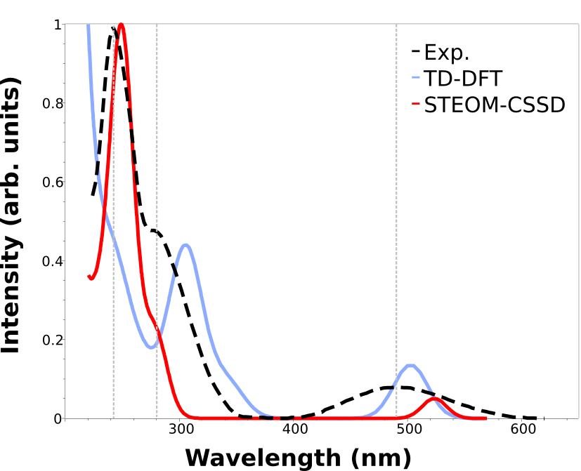
Here we added the gray vertical lines to guide the eye to the first three peaks of the spectrum. As you can see, although TD-DFT works well to predict the first, the higher energy ones are largely displaced.
That can happen when these states are significantly different, and the associated error is not comparable. One advantages of the STEOM is that there is a more balanced treatment of different excited states and such situations and avoided.
The calculated results are now well in line with the experiment through the whole spectrum, except for a small deviation on the intensities. We can arrange these results in a table to facilitate visualization: below there is comparison of the energy error of the first three peaks measured for the E isomer. The TD-DFT can be as high as 1 eV!
| Peak | TD-DFT | STEOM | Exp. |
|---|---|---|---|
| 1 | 4.23 | 5.06 | 5.14 |
| 2 | 3.83 | 4.42 | 4.43 |
| 3 | 2.46 | 2.45 | 2.53 |
Even if the predicted spectrum matches the experiment, the calculation is still not reproducing exactly what happens during light absorption. The full experimental spectra must also include vibrational resolution, and maybe even vibronic coupling. That can be included with the ORCA_ESD module.