Gromacs模拟介电屏蔽
教程来源:Dielectric screening | MD Simulation Techniques and Applications (psu.edu)
github: Zuttergutao/Gromacs-Tutorials (github.com)
前言
离子微扰水层结构
笔者对于此教程涉及的一些理论并不精通,甚至完全不懂。写(翻译)此教程的目的也是发现其模拟的protocol很有意思。如果有理论或者专业术语使用不正确的地方,欢迎批评指正!
溶液中的离子从立体和静电角度扰乱了附近水分子的排列。 离子占据了空间,这本身就导致了附近水分子的非均匀浓度分布,离子本身有一个排斥半径和有一个近邻的外壳层,当局部浓度弛豫到其平均值时,会出现衰减的振荡。 对于离子电荷附近的水分子的排布,像Na+这样的正离子倾向于吸引带负电的氧原子,排斥水面上带正电的氢原子。
静电势也同样因离子的存在而受到扰乱。 在真空中,离子会有一个库伦场,以$\frac{1}{r^2}$的速度衰减。 在水中,附近水分子的定向偶极子倾向于屏蔽离子的场,因为带相反电荷的原子聚集在离子周围的壳层中,从而平衡体系电荷。
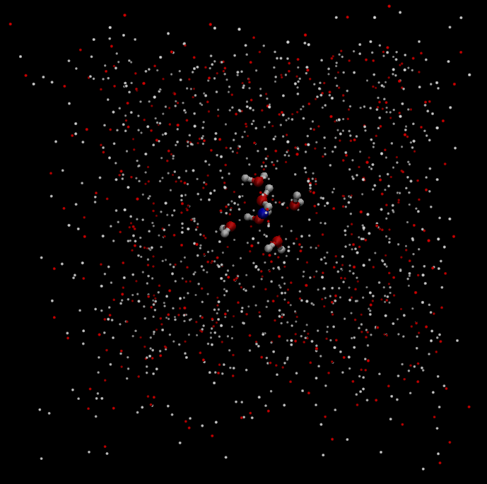
我们可以使用MD来探索水在离子附近的这种屏蔽行为。通过将一个Na+离子固定在水盒子的中心,使用模拟轨迹计算平均电场、偶极方向、电荷密度和固定离子附近的分子分布。
模拟
构建和平衡体系
体系为水盒子中含有一个Na+离子。首先创建一个gro文件,将Na+离子摆放在2.5*2.5*2.5 nm盒子正中央,然后使用gmx solvate给体系添加水。接着就是能量最小化、100 ps NVT和100 ps NPT,步长取2 fs。在模拟期间,Na+离子必须被冻结。使用oplsaa力场
-
创建Na+离子gro文件。
# Na.gro1
2
3
4Na ion
1
1NA NA 1 1.250 1.250 1.250
2.50000 2.50000 2.50000 -
溶剂化盒子(记住加了多少水分子)
1
gmx solvate -cp Na.gro -o system.gro -box 2.5 2.5 2.5
-
构建topol (此例使用oplsaa力场)
# topol.top1
2
3
4
5
6
7
8
9
10
11
12#include "oplsaa.ff/forcefield.itp"
#include "oplsaa.ff/ions.itp"
#include "oplsaa.ff/spce.itp"
[ system ]
; Name
Na+ in water
[ molecules ]
; Compound #mols
NA 1
SOL 509 ; 填入相应的水分子数 -
EM
#em.mdp1
2
3
4
5
6
7
8
9
10
11
12
13
14
15
16
17
18
19
20
21
22
23
24
25
26
27
28
29define = -DFLEXIBLE
; Run control
integrator = steep
nsteps = 5000
; EM criteria and other stuff
emtol = 100
emstep = 0.01
; Output control
nstlog = 10
nstenergy = 10
; cutoffs
cutoff-scheme = verlet
nstlist = 20
ns_type = grid
pbc = xyz
rlist = 1.0
coulombtype = PME
rcoulomb = 1.0
vdwtype = cutoff
rvdw = 1.0
; Temperature and pressure coupling are off during EM
tcoupl = no
pcoupl = no
freezegrps = Ion
freezedim = Y Y Y1
2gmx grompp -f em.mdp -c system.gro -p topol.top -o em.tpr -maxwarn 5
gmx mdrun -v -deffnm em -nt 1 -
NVT
#nvt.mdp1
2
3
4
5
6
7
8
9
10
11
12
13
14
15
16
17
18
19
20
21
22
23
24
25
26
27
28
29
30
31
32
33
34
35
36
37
38
39
40
41; Run control
integrator = md
tinit = 0
dt = 0.002
nsteps = 50000 ; 100ps
; Output control
nstxout = 500
nstlog = 500
nstenergy = 500
; cutoffs
cutoff-scheme = verlet
nstlist = 20
ns_type = grid
pbc = xyz
rlist = 1.0
coulombtype = PME
rcoulomb = 1.0
vdwtype = cutoff
rvdw = 1.0
; Temperature coupling
tcoupl = v-rescale
tc_grps = system
tau_t = 0.1
ref_t = 300
; Pressure coupling is off for NVT
Pcoupl = No
tau_p = 0.5
compressibility = 4.5e-05
ref_p = 1.0
; Generate velocities to start
gen_vel = yes
gen_temp = 300
gen_seed = -1
freezegrps = Ion
freezedim = Y Y Y1
2gmx grompp -f nvt.mdp -c em.gro -p topol.top -o nvt.tpr -maxwarn 5
gmx mdrun -v -deffnm nvt -nt 4 -
NPT
#npt.mdp1
2
3
4
5
6
7
8
9
10
11
12
13
14
15
16
17
18
19
20
21
22
23
24
25
26
27
28
29
30
31
32
33
34
35
36; Run control
integrator = md
tinit = 0
dt = 0.002
nsteps = 50000 ; 100ps
; Output control
nstxout = 500
nstlog = 500
nstenergy = 500
; cutoffs
cutoff-scheme = verlet
nstlist = 20
ns_type = grid
pbc = xyz
rlist = 1.0
coulombtype = PME
rcoulomb = 1.0
vdwtype = cutoff
rvdw = 1.0
; Temperature coupling
tcoupl = v-rescale
tc_grps = system
tau_t = 0.1
ref_t = 300
; Pressure coupling
Pcoupl = berendsen
tau_p = 0.5
compressibility = 4.5e-05
ref_p = 1.0
freezegrps = Ion
freezedim = Y Y Y1
2gmx grompp -f npt.mdp -c nvt.gro -p topol.top -o npt.tpr -maxwarn 5
gmx mdrun -v -deffnm npt -nt 4 -
Prod
# run.mdp1
2
3
4
5
6
7
8
9
10
11
12
13
14
15
16
17
18
19
20
21
22
23
24
25
26
27
28
29
30
31
32
33
34
35
36
37
38; Run control
integrator = md
tinit = 0
dt = 0.002
nsteps = 500000 ; 1 ns
; Output control
nstxout = 500
nstvout = 500
nstfout = 500
nstlog = 5000
nstenergy = 500
; cutoffs
cutoff-scheme = verlet
nstlist = 20
ns_type = grid
pbc = xyz
rlist = 1.0
coulombtype = PME
rcoulomb = 1.0
vdwtype = cutoff
rvdw = 1.0
; Temperature coupling
tcoupl = v-rescale
tc_grps = system
tau_t = 0.1
ref_t = 300
; Pressure coupling
Pcoupl = berendsen
tau_p = 0.5
compressibility = 4.5e-05
ref_p = 1.0
freezegrps = Ion
freezedim = Y Y Y1
2gmx grompp -f run.mdp -c npt.gro -p topol.top -o run.tpr -maxwarn 5
gmx mdrun -v -deffnm run -nt 4
添加测试电荷并MD
如何往体系中添加测试电荷?
首先,修改top文件,修改选中水分子的定义,复制oplsaa.ff/scpe.itp(水的力场topol文件)到运行文件夹并重命名为spceq.itp;修改水分子名为SOLq,氧原子带一个单位正电荷。最后,移除SETTLES申明(topol中只允许申明一组SETTLES,在spce.itp中已经申明了一组)。
-
spceq.itp1
2
3
4
5
6
7
8
9
10
11
12
13
14
15
16
17
18
19[ moleculetype ]
; molname nrexcl
SOLq 2
[ atoms ]
; nr type resnr residue atom cgnr charge mass
1 opls_116 1 SOL OW 1 0.1524 ; overridden charge
;1 opls_116 1 SOL OW 1 -0.8476 ; original parameters
2 opls_117 1 SOL HW1 1 0.4238
3 opls_117 1 SOL HW2 1 0.4238
[ bonds ]
; i j funct length force.c.
1 2 1 0.1 345000 0.1 345000
1 3 1 0.1 345000 0.1 345000
[ angles ]
; i j k funct angle force.c.
2 1 3 1 109.47 383 109.47 383 -
修改topol.top,并命名为
systemq0.top此文件为模板文件。在后续随机选定带电水分子时被使用。
通过后文描述的脚本,将NTOP和NBOT值替换。
1
2
3
4
5
6
7
8
9
10
11
12
13
14
15#include "oplsaa.ff/forcefield.itp"
#include "oplsaa.ff/ions.itp"
#include "oplsaa.ff/spce.itp"
#include "spceq.itp"
[ system ]
; Name
H2O
[ molecules ]
; Compound #mols
NA 1
SOL NTOP
SOLq 1
SOL NBOT同时创建一个ndx模板文件,在最后添加如下行。
脚本将会将OW,HW1,HW2替换为选中水分子的原子index,用于后续分析。
#systemq.ndx1
2[ testq ]
OW HW1 HW2 -
Loop over molecules
1
2
3
4
5
6
7
8
9
10
11
12
13
14
15
16
17
18
19
20
21
22
23
24
25
26
27
28
29
30
31
32
33
34
35
36
37
38
39
40
41
42
43
44
45
46
47
48cd ..
dir=$PWD
cd loop
SYSTEM=$dir/System
MDP=$dir/MDP
INIT=$dir/MD/run/run.gro
# generate random number between 2 and 508 inclusive
let Y=508
let X=2
BASE=$((Y-X+1))
# loop over randomly chosen water molecules
let K=1
let KMAX=500
while (($K < $KMAX))
do
# randomly select test molecule
NTOP=$(($(($RANDOM%$BASE))+X))
let NBOT=508-${NTOP}
sed "s/NTOP/${NTOP}/;s/NBOT/${NBOT}/" < $SYSTEM/systemq0.top > $SYSTEM/systemq.top
# create index file with test molecule
let OW=1+3*${NTOP}+1
let HW1=${OW}+1
let HW2=${OW}+2
sed "s/OW/${OW}/;s/HW1/${HW1}/;s/HW2/${HW2}/" < $SYSTEM/systemq.ndx > systemq.ndx
# rerun without test charge
gmx grompp -f $MDP/run.mdp -c $INIT -p $SYSTEM/topol.top -n systemq.ndx -o rerun.tpr -maxwarn 20
gmx mdrun -nt 1 -deffnm rerun -rerun run.trr
# force without test charge
echo "7" | gmx traj -f rerun.trr -s rerun.tpr -n systemq.ndx -com -of force_${K}.xvg
# rerun with test charge
gmx grompp -f $MDP/run.mdp -c $INIT -p $SYSTEM/systemq.top -n systemq.ndx -o rerunq.tpr -maxwarn 20
gmx mdrun -nt 1 -deffnm rerunq -rerun run.trr
# force with test charge
echo "7" | gmx traj -f rerunq.trr -s rerunq.tpr -n systemq.ndx -com -of forceq_${K}.xvg
# test molecule atom positions (for dipole, charge distrib,...)
echo "7" | gmx traj -f rerunq.trr -s rerunq.tpr -n systemq.ndx -ox posn_${K}.xvg
rm "#"*"#"
let K=$K+1
done用户脚本将执行如下操作
- 随机选择水分子
- 使用
sed "s/NTOP/${NTOP}/;s/NBOT/${NBOT}/" < $SYSTEM/systemq0.top > $SYSTEM/systemq.top命令从模板systemq0.top生成systemq.top - 使用
sed "s/OW/${OW}/;s/HW1/${HW1}/;s/HW2/${HW2}/" < $SYSTEM/systemq.ndx > systemq.ndx命令从模板systemq.ndx生成systemq.ndx文件 - 不带电荷重新运行已经存在的轨迹,输出选中水分子的力
- 带电荷重新运行已经存在的轨迹,输出选中水分子的力
- 删除backup文件
KMAX表示运行多少次,在此设置的是500.生成随机数:系统变量
RANDOM会返回0-32767范围内的随机整数。使用如下命令生成X-Y区间内的随机整数R
%为取余算符1
2BASE=$((Y-X+1))
R=$(($(($RANDOM%$BASE))+X))替换规则:一共有NTOTAL个水分子,其中NTOP范围为1~(NTOTAL-2),NBOT范围为(NTOTAL-1 ~ NTOP)。随机选取了一个水分子之后,NTOP即确定下来,那么选中水分子的原子index:{OW:1+3*NTOP+1},{HW1:1+3*NTOP+2},{HW:1+3*NTOP+1}。其中第一个1为Na离子,3*NTOP为NTOP个水分子的原子数目。
rerun
1
2
gmx grompp -f run.mdp -c run.gro -p systemq.top -n systemq.ndx -o rerunq.tpr -maxwarn 20
gmx mdrun -nt 1 -deffnm rerunq -rerun run.trr重新运行轨迹的目的:通过新生成的tpr文件重新计算力和能量,但是原子还是按原有轨迹运动。
write force,position
使用
gmx traj命令输出选中原子的位置或者力到xvg文件选中group 7,输出group的质心力,
-of指定力的输出文件。1
echo “7” | gmx traj -f rerunq.trr -s rerunq.tpr -n systemq.ndx -com -of forceq_${K}.xvg
分析
因为gromacs并没有计算电荷力与分子排布的分析程序,原教程中使用mathematica进行分析,如果有会使用此软件的,可以打开提供的网址下载相关文件进行测试。在此,使用python进行分析(在文末给出完整python代码)
使用环境:python
包:
- numpy
- matplotlib
数据处理
-
导入数据
1
2
3
4
5
6
7
8
9# 导入未加电荷的force文件
forcedata=[]
for i in range(num):
forcefile="force_"+str(i+1)+".xvg"
with open(forcefile) as f:
lines=f.readlines()
tmp=np.array([[float(i) for i in l.split()] for l in lines[26:]])[:,1:]
forcedata.append(tmp)
forcedata=np.array(forcedata)上述代码读取每个模拟时测试水分子为添加电荷的力输出文件,并删除第一列模拟时间。通过带电force文件与不带电force文件相减获得力差数组。其余输入文件的处理方式与上述代码相近。
-
位移向量与距离
1
2
3
4
5
6
7
8
9
10
11
12
13
14
15
16
17
18
19
20# Separation vectors and distances
# 计算O原子、H原子和电荷中心的位置、单位向量和相对于Na离子的距离
# Na离子在盒子中心
lBox=2.5
boxCtr=[lBox/2,lBox/2,lBox/2]
# 距离盒子中心的Vec
# 通过mod with offset 将体系周期性保留
# ctrVec=(opositions-boxCtr)-3*np.floor(((opositions-boxCtr)+lBox/2)/lBox)
def ctrVec(m):
return (m-boxCtr)-lBox*np.floor(((m-boxCtr)+lBox/2)/lBox)
# 距离盒子中心的最近距离
def ctrDist(m):
return np.linalg.norm(ctrVec(m),axis=1).reshape(np.linalg.norm(ctrVec(m),axis=1).shape[0],1)
# 距离盒子中心的单位矢量
def ctrUnit(m):
return ctrVec(m)/ctrDist(m)计算所有O原子、H原子和电荷中心(COC)的位移向量和距离。在计算中,考虑周期性边界条件,计算出最短的位移向量。在周期为L的周期系统中,最短位移向量的分量范围为{-L/2, L/2}。要计算最短的位移向量,一个有用的函数是Mod[r, L, -L/2],它返回其参数映射到长度为L的区间,但移动了-L/2,即映射到{-L/2,L/2}。该函数为带有偏移量的模余算法(参考链接:Modulo - Wikipedia)
在进行绘制之前,我们需要对原子位置数据进行格式化。
1
2
3
4
5
6
7
8
9
10
11opositions=posndata[:,:,0,:]
hpositions=posndata[:,:,1:3,:]
cpositions=0.5*posndata[:,:,0,:]+0.25*posndata[:,:,1,:]+0.25*posndata[:,:,2,:]
cpositions=cpositions.reshape(cpositions.shape[0]*cpositions.shape[1],3)
opositions=opositions.reshape(opositions.shape[0]*opositions.shape[1],3)
hpositions=hpositions.reshape(hpositions.shape[0]*hpositions.shape[1]*hpositions.shape[2],3)
unitVecsO=ctrUnit(opositions)
unitVecsC=ctrUnit(cpositions)
rValueC=ctrDist(cpositions)
rValueH=ctrDist(hpositions)
rValueO=ctrDist(opositions)
计算和绘制偶极子
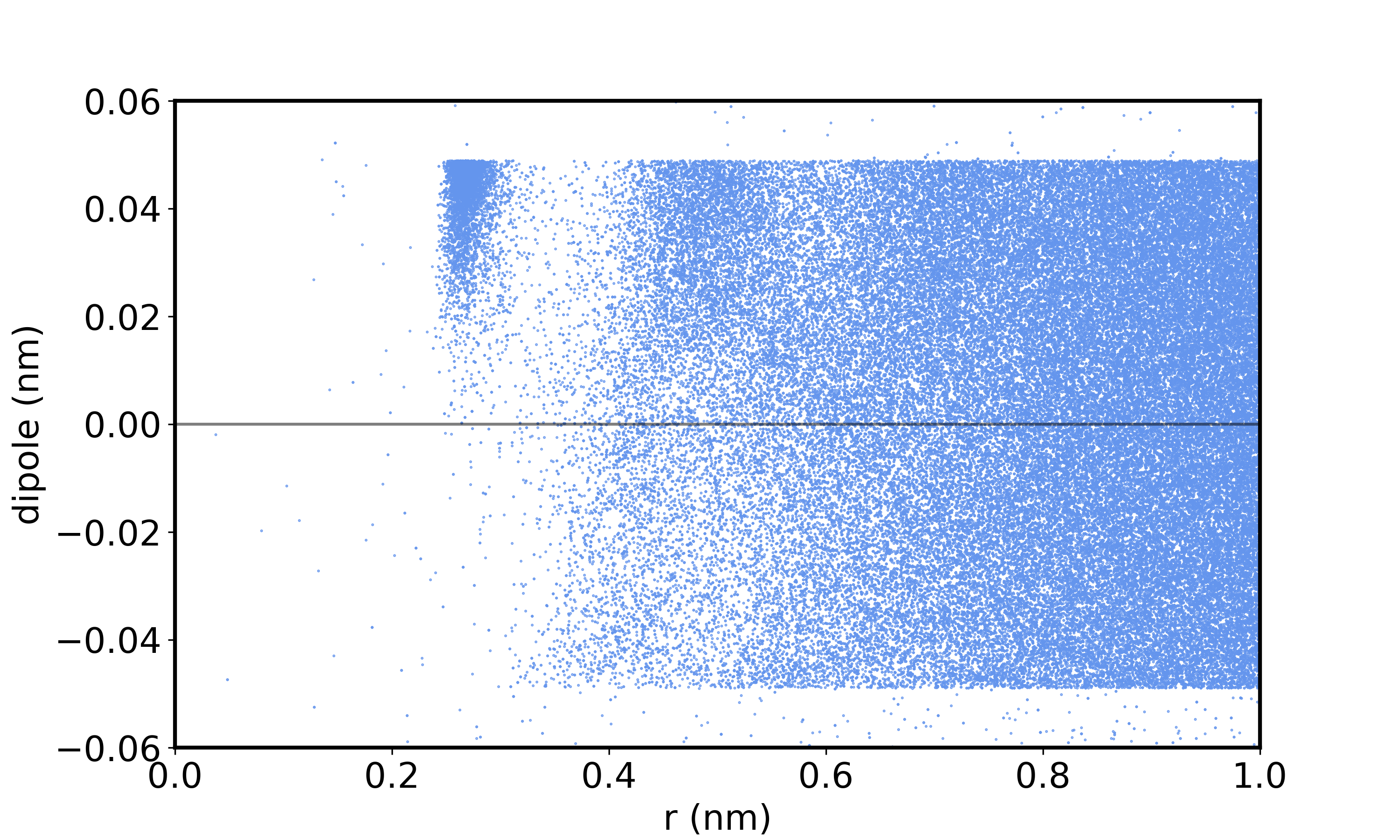
使用原子位置计算偶极子;
沿单位矢量从Na+中心到电荷中心的偶极子。做一个散点图的偶极子分量沿矢量到盒中心,与距离盒中心。
如图所示,在距离Na+离子中心3A处的邻近壳层中,有强取向偶极子。远离离子,偶极子分量沿分离矢量是随机的,均匀分布在-0.05到0.05。
计算和绘制力
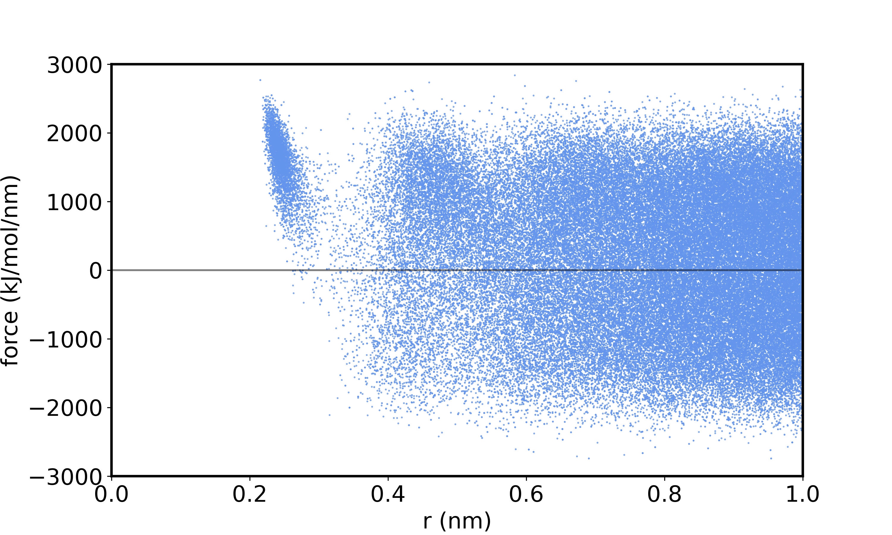
沿着从Na+中心到测试电荷(氧原子)的单位矢量投影带电和不带电测试分子之间的力差值。
图3显示了距离Na+离子中心约3A处邻近壳层的强定向库仑力。
平均力vs距离

对于半径范围[xmin,xmax]取nx等分,对于这nx区间内的force取平均值,绘制不同区间内力与距离的关系。类似地,也将此过程应用到偶极与电荷上。
图中绘制了(正)单元测试电荷(+1电荷添加到随机选择的水分子中的氧原子上)上的平均力与距离的关系图。该力是排斥性的,并随距离衰减;振荡是由与近邻壳中的诱导偶极子相互作用引起的。
平均偶极子vs距离
平均偶极子在邻近壳层很强,随着与Na+离子的距离而衰减,并显示了对应于相邻壳层的振荡。最大偶极投影(因此水分子的偶极矩)约为0.5 eA,因此最靠近Na+离子的偶极几乎完全定向。
平均电荷vs距离
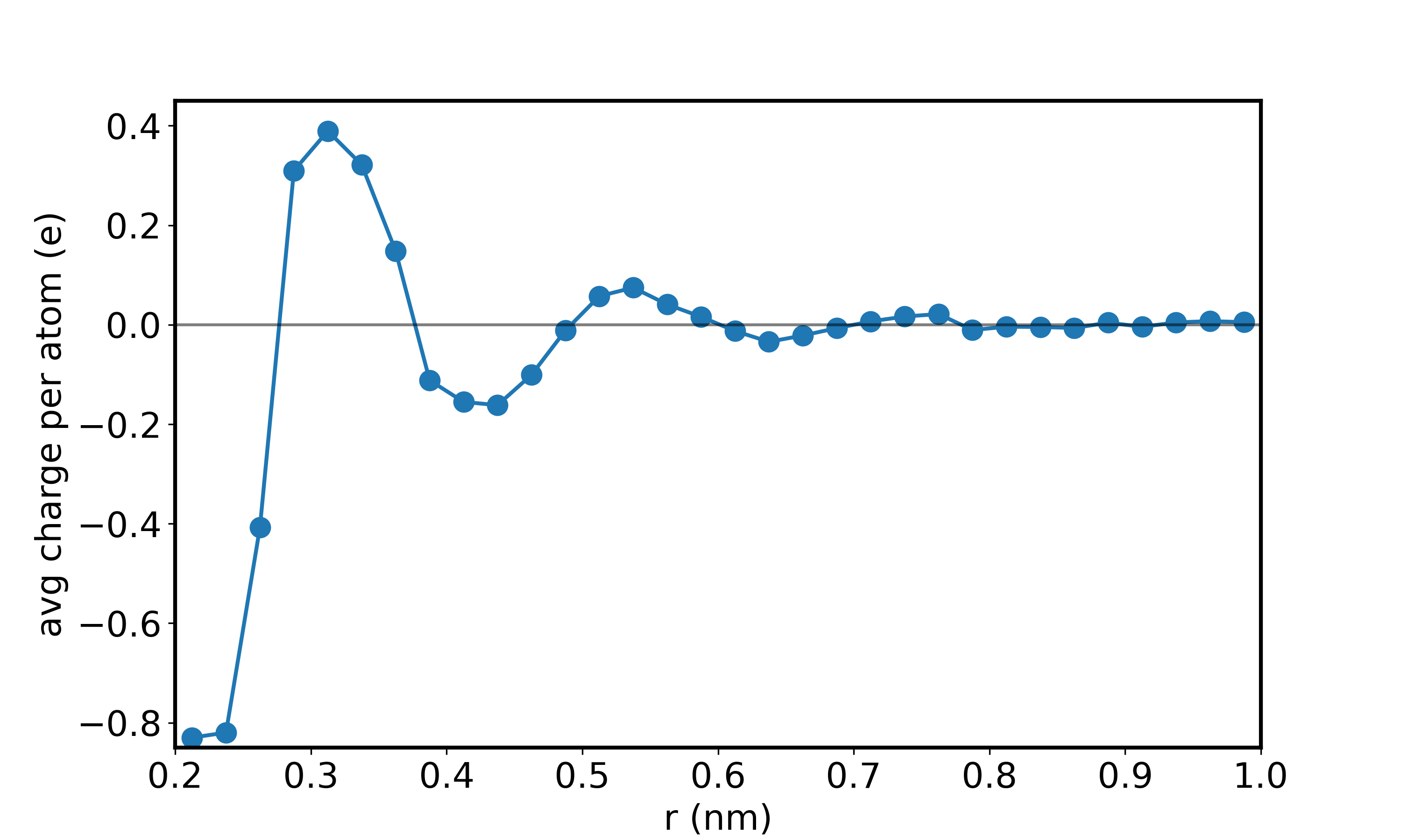
计算存在的每个原子的平均电荷与到盒子中心的距离。
图 6 显示每个原子的平均电荷在 Na+ 离子附近呈强负性;这反映了近邻壳层中定向水偶极子的氧“头”的存在,其点电荷为 -0.8476。稍远一点,每个原子的电荷为正,对应于定向近邻偶极子的氢“尾巴”,其点电荷为 +0.4238。
Na-O、Na-H相关函数
.png)
.png)
我们可以从 O 和 H 原子到盒子中心的距离数据中计算 O 和 H 原子的平均密度。本质上是 Na-O 和 Na-H 径向分布函数。
电荷密度与距离
.png)
最后绘制电荷密度与距离的分布图
图显示了由此产生的电荷密度,它表现出强烈的负峰和正峰,对应于近邻壳层中强取向的偶极子,然后是弱和扩散的第二邻峰。
代码
1 | import numpy as np |